How do artificial neural networks learn complex patterns directly from examples rather than handwritten rules? This accessible synthesis review traces the evolution from early perceptrons and backpropagation to CNNs, LSTMs, Transformers, and Graph Neural Networks, explaining in plain language how network wiring matches data geometry, why residual connections and normalization stabilize deep training, and how phenomena like double descent challenge classical statistical intuition.
Introduction: Learning by Example Instead of Writing Rules
For decades, most computer software worked like a detailed recipe: human programmers had to anticipate every edge case and write explicit if-then instructions by hand. That strategy works well for accounting or sorting spreadsheets, but it breaks down on everyday perceptual tasks—recognizing a face in dim light, transcribing spoken words over background noise, or predicting how a chain of amino acids will fold into a three-dimensional protein. There are simply too many subtle variations to specify with handwritten rules.
Artificial neural networks flip this paradigm around. Instead of programming the rules directly, researchers design a flexible network of simple connected processing units—loosely inspired by biological neurons—and let the system adjust its own internal connection strengths ("weights") by studying thousands or millions of examples (LeCun et al., 2015). This synthesis reviews how neural networks evolved from simple binary switches into modern deep learning systems, how different network designs suit different kinds of data, why training them works better than early theory predicted, and how they are reshaping modern science.
A Brief History: Three Waves of Neural Network Research
Wave 1: The Perceptron and Early Linear Limits
The story begins in the late 1950s with Frank Rosenblatt's Perceptron (Rosenblatt, 1958). A perceptron takes a list of numerical inputs, multiplies each input by a learned weight representing its importance, adds them up, and fires a yes-or-no output if the total crosses a threshold. Rosenblatt proved a celebrated result: whenever two categories can be separated by a clean straight boundary (like separating tall, heavy objects from short, light ones on a chart), a simple error-correction loop will reliably find that separating line.
The catch, however, soon cooled early enthusiasm: a single layer of threshold units can only draw straight boundaries. Whenever a problem requires combining clues interactively—for instance, recognizing when two conditions agree or differ—a flat one-layer perceptron gets stuck. Solving richer problems required stacking multiple hidden layers of neurons between the input and the final answer.
Wave 2: Energy Landscapes and Backpropagation
Two conceptual leaps revived the field in the 1980s. First, physicist John Hopfield showed that networks with feedback connections—now known as Hopfield networks—behave like physical systems settling into low-energy valleys, much like a marble rolling to the bottom of a bowl, enabling memories to be retrieved from partial or noisy clues (Hopfield, 1982), closely echoing ideas from the Boltzmann distribution in statistical physics. Second, David Rumelhart, Geoffrey Hinton, and Ronald Williams popularized backpropagation (Rumelhart et al., 1986): a systematic way to assign credit or blame backward through a multi-layer network so every hidden neuron learns from the final mistake.
Shortly afterward, mathematical proofs showed that even a relatively simple two-layer network with smooth S-shaped activations can, in principle, approximate virtually any continuous input-output relationship given enough hidden neurons (Cybenko, 1989; Hornik et al., 1989). Yet theory and practice initially diverged: training deep multi-layer networks remained slow and finicky, pushing researchers toward alternative methods like support vector machines throughout the 1990s.
Wave 3: Depth, GPUs, and Large-Scale Pretraining
Everything changed in the late 2000s and early 2010s as three forces converged: massive labeled datasets, graphics processors (GPUs) capable of fast parallel matrix math, and architectural refinements that kept training signals stable across many layers (Hinton & Salakhutdinov, 2006). When Alex Krizhevsky and colleagues trained a deep convolutional network on over a million images in 2012, error rates plummeted nearly in half compared to hand-engineered computer vision pipelines (Krizhevsky et al., 2017)—launching the modern deep learning era.
How a Neural Network Actually Learns
Layers, Nonlinearity, and Building Concepts Step by Step
At its core, a neural network passes data through a sequence of simple stages, often called layers. Each neuron computes a weighted blend of incoming signals plus an offset ("bias"), and then passes the result through a simple nonlinear activation function—most commonly a ReLU filter that keeps positive numbers intact and sets negative numbers to zero.
That tiny nonlinear gate is essential. Without it, stacking ten linear layers together mathematically collapses into a single flat equation, giving the network no more expressive power than one layer. With nonlinear gates between layers, each stage warps and folds the data step by step: early layers spot simple local clues (like edges in a photo or short motifs in a DNA sequence), middle layers assemble those clues into parts (eyes, wheels, binding pockets), and later layers combine parts into whole concepts—turning tangled raw data into cleanly separated internal maps, or neural manifolds.
Measuring Mistakes and Walking Downhill
Before training starts, a network's weights are initialized near random values, so its first guesses are poor. Learning works through a four-step feedback loop:
- Forward Pass: Data moves layer by layer from input to output to produce a prediction.
- Loss Function Score: A scoring rule—such as prediction error for numbers or Kullback–Leibler (KL) divergence / cross-entropy for probabilities—measures how far the guess landed from the known answer.
- Backward Pass (Backpropagation): Using the chain rule of calculus, the network traces backward from the output to figure out whether nudging each individual weight slightly up or down would shrink the error.
- Parameter Update (Gradient Descent): An optimizer steps every weight a small distance downhill toward lower error, repeating across millions of training examples.
A helpful everyday analogy is adjusting the temperature of a shower when multiple pipes and valves interact downstream: once you feel whether the water is too hot or too cold, you trace backward along the plumbing to turn each upstream valve a tiny fraction in the direction that improves comfort, rather than twisting valves blindly.
Major Network Architectures and Why Structure Matters
One of the clearest lessons from deep learning literature is that network wiring is not one-size-fits-all. A naive network where every neuron connects to every pixel or word wastes millions of weights rediscovering basic geometry from scratch. Instead, successful architectures build helpful structural assumptions—often called inductive biases—directly into their layout (Table 1).
| Architecture | Plain-Language Intuition | Key Strength | Main Limitation | Landmark Literature |
|---|---|---|---|---|
| Feedforward Network (MLP) | Every neuron in one layer talks to every neuron in the next | Flexible general-purpose approximator for tabular or coordinate data | Scales poorly on raw images or long sequences without structural priors | Rumelhart et al., 1986; Hornik et al., 1989 |
| Convolutional Network (CNN) | Small pattern detectors slide across an image or grid | Recognizes a motif anywhere in the scene with very few parameters | Less natural for irregular networks or very long-range context | LeCun et al., 1998; Krizhevsky et al., 2017; Rawat & Wang, 2017 |
| Residual Network (ResNet) | Adds a direct bypass lane around groups of layers | Allows 100+ layers to train cleanly without losing gradient signals | Still relies on the underlying layer type for spatial or sequence priors | He et al., 2016 |
| Gated Recurrent Net (LSTM / RNN) | Reads a stream one step at a time while updating an internal scratchpad | Naturally handles live streaming audio, sensors, or variable lengths | Harder to parallelize during training; memory can fade over thousands of steps | Hochreiter & Schmidhuber, 1997 |
| Transformer (Self-Attention) | Every word or token directly weighs which other tokens matter most right now | Captures long-distance relationships in one step and scales smoothly on GPUs | Memory cost grows rapidly on extremely long sequences | Jumper et al., 2021 (AlphaFold) |
| Graph Neural Network (GNN) | Connected nodes exchange summary messages with their immediate neighbors | Respects arbitrary shapes like chemical bonds or social graphs regardless of node numbering | Can blur local details if too many message rounds average everything together | Scarselli et al., 2009 |
Convolutional Networks for Spatial Data
In images, audio spectrograms, and microscopy scans, nearby pixels belong together, and an edge or cell looks essentially the same whether it sits in the upper-left corner or near the center. Convolutional Neural Networks (CNNs) capitalize on both facts by scanning small shared filters across the entire grid (LeCun et al., 1998; Rawat & Wang, 2017). Because every location reuses the same filter weights, a CNN generalizes automatically across positions while keeping memory requirements dramatically smaller than fully connected networks (Krizhevsky et al., 2017).
Recurrent Networks and Gated Memory
When data unfolds over time—such as spoken sentences, ECG heartbeats, or neural recordings—Recurrent Neural Networks (RNNs) maintain a running summary of everything seen so far. Early RNNs struggled because error signals shrank or blew up as they were multiplied step after step backward through time. The Long Short-Term Memory (LSTM) design (Hochreiter & Schmidhuber, 1997) solved much of this decay by adding explicit learnable gates—like control valves—that decide what information to keep, update, or clear from long-term memory.
Transformers and Self-Attention
Transformers replaced step-by-step recurrence with self-attention. Instead of passing memories sequentially down a chain of time steps, every item in a sequence compares itself against every other item simultaneously and pulls in context from whichever neighbors are most relevant—much like a reader scanning a sentence to immediately link a pronoun back to a noun three clauses earlier. Because these comparisons run in parallel across modern hardware, Transformers unlocked massive foundation models in text, vision, and biological sequence modeling such as AlphaFold (Jumper et al., 2021).
Graph Neural Networks for Molecules and Networks
Molecules, metabolic pathways, and ecological food webs do not live on neat camera grids or straight lines—they are flexible webs of relationships. Graph Neural Networks mirror that geometry directly: each atom or node gathers information from its bonded neighbors, updates its internal state, and repeats across several rounds (Scarselli et al., 2009), guided by the overall network connectivity captured by tools such as the graph Laplacian.
Making Deep Networks Trainable and Reliable
Designing a promising architecture is only half the battle; deep networks historically stalled or diverged unless signals stayed well-behaved across dozens of layers. Modern deep learning relies on several practical stabilization breakthroughs (Table 2).
| Technique | Problem Solved | How It Works in Plain Terms | Practical Impact |
|---|---|---|---|
| Non-Saturating Activations (ReLU, GELU) | Vanishing learning signals through flat S-curves | Keep slopes responsive across positive inputs instead of squashing everything between 0 and 1 | Allowed networks deeper than 3-4 layers to converge quickly |
| Skip / Residual Connections | Accuracy degrading as networks get very deep | Let each block learn a gentle adjustment added onto an unchanged copy of its input (He et al., 2016) | Made 50- to 1,000-layer networks routine and dependable |
| Layer & Batch Normalization | Internal signals drifting wildly as weights update | Re-center and re-scale numbers inside each layer to stay in a steady numerical sweet spot | Smooths optimization and allows larger learning steps |
| Adaptive Optimizers (SGD + Momentum, AdamW) | Slow progress in narrow valleys & noisy mini-batches | Build rolling velocity downhill and scale step sizes per weight while gently shrinking oversized weights | Trains billion-parameter models without costly second-derivative matrices |
Why First-Order Steps Beat Classical Second-Order Methods at Scale
In small engineering problems, classical optimization techniques like Newton's method or BFGS use curvature information to leap straight toward the bottom of a bowl in just a few steps. On a neural network with millions or billions of weights, however, storing that full curvature table is impossible. Deep learning instead uses small, noisy mini-batches of examples with enhanced gradient descent—trading exact curvature for rapid, cheap steps whose gentle randomness actually helps bounce training out of dead-end plateaus.
Rethinking Overfitting: High-Dimensional Landscapes and Double Descent
Two theoretical surprises have reshaped how scientists think about neural learning. First, early critics worried deep networks would get trapped in poor "local minima" valleys. In ultra-high dimensions, however, almost all high-error flat spots turn out to be saddle points—shapes curved upward in some directions and downward in others, like a mountain pass—so noisy mini-batch updates naturally slide off toward good solutions.
Second, classical statistics taught that giving a model more parameters than training examples causes memorization and poor generalization (overfitting). Remarkably, modern neural networks follow a double-descent pattern (Belkin et al., 2019): accuracy initially worsens right where parameter count matches dataset size, but then improves again when models grow far larger than the dataset, because gradient descent naturally favors smooth, low-complexity solutions among all ways to fit the training points.
Transformative Impact Across Science and Open Challenges
From Perceptual Benchmarks to Scientific Discovery
Originally built for recognizing handwritten digits (LeCun et al., 1998) and sorting photographs (Krizhevsky et al., 2017), neural networks have become core scientific instruments. In structural biology, AlphaFold combined evolutionary sequence alignments with attention over 3D residue pairs to predict protein structures at near-experimental accuracy (Jumper et al., 2021). In chemistry and neuroscience, molecular GNNs accelerate catalyst and drug screening, while latent representation models uncover low-dimensional brain dynamics in neural decoding and neural manifold studies—complementing classical Bayesian inference and information-theoretic analysis.
Persistent Limits and Research Frontiers
Despite dramatic empirical progress, major scientific limitations remain active frontiers in the literature:
- Distribution Shift & Extrapolation: Standard networks interpolate reliably inside regimes resembling their training data, but predictions can fail abruptly when experimental conditions shift out of distribution.
- Calibration & Uncertainty: Deep classifiers can produce overconfident probabilities on unfamiliar inputs unless paired with Bayesian ensembles or conformal calibration.
- Interpretability & Physical Guarantees: Ensuring learned surrogates respect exact conservation laws (energy, mass, symmetry) and exposing human-understandable mechanisms remains essential for high-stakes scientific deployment.
- Data, Energy & Compute Footprints: Frontier pretraining consumes substantial compute and curated data, motivating sparser architectures, data-efficient transfer learning, and specialized domain priors.
Interactive 3D Exploration in NeuroSpace Lab
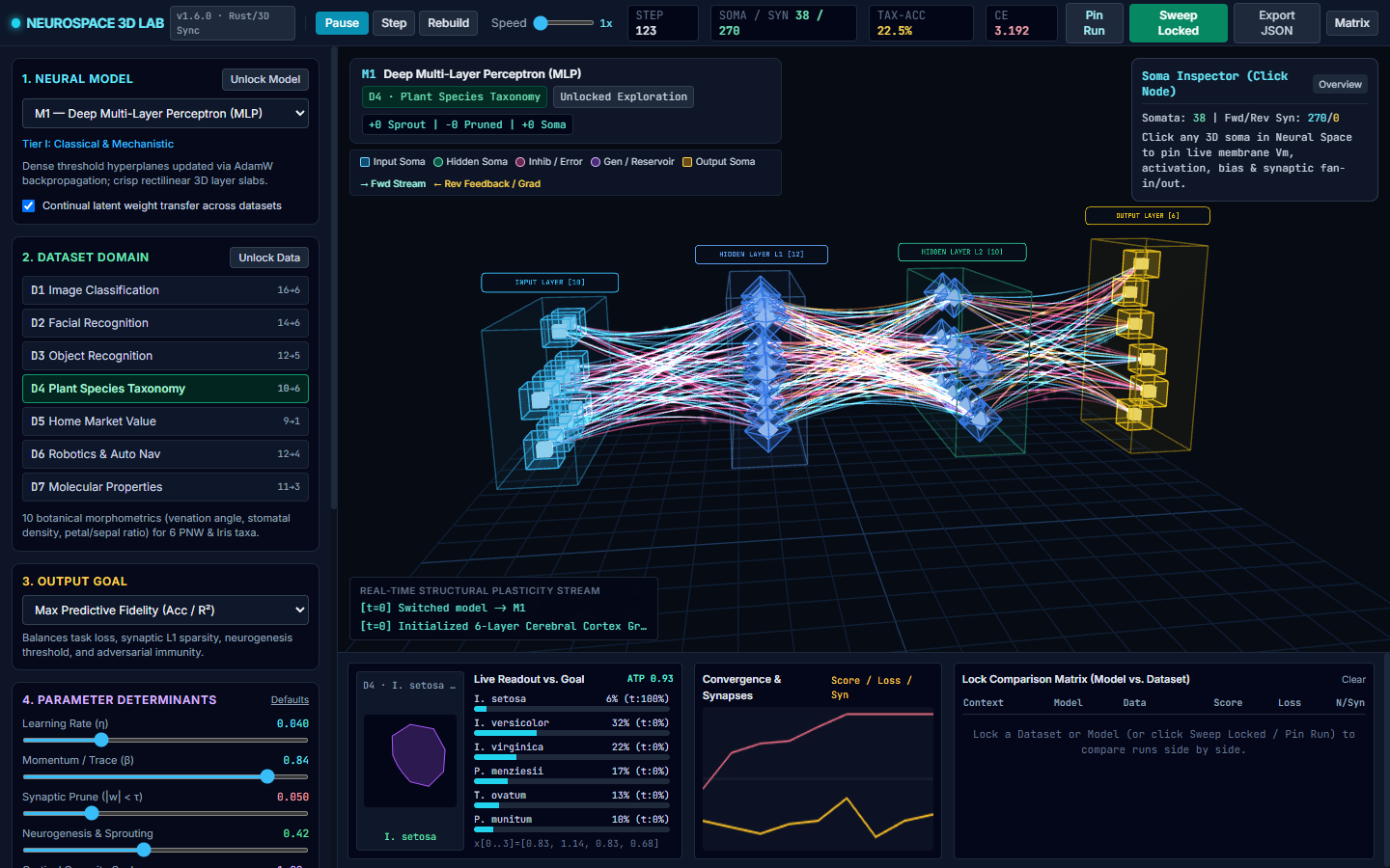
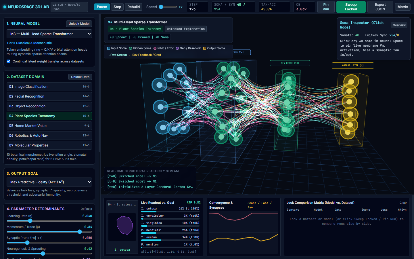
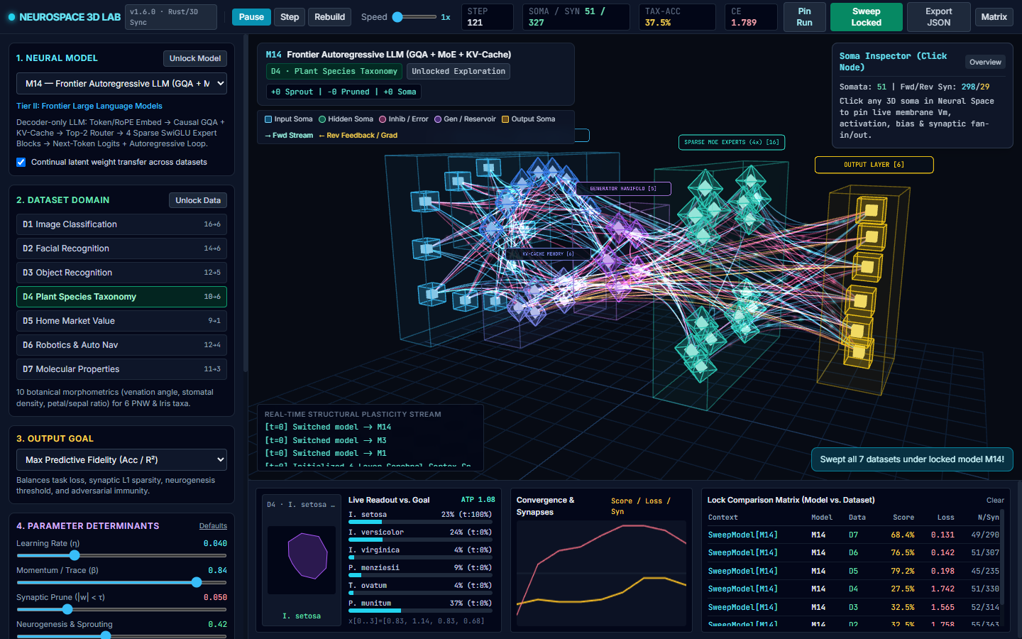
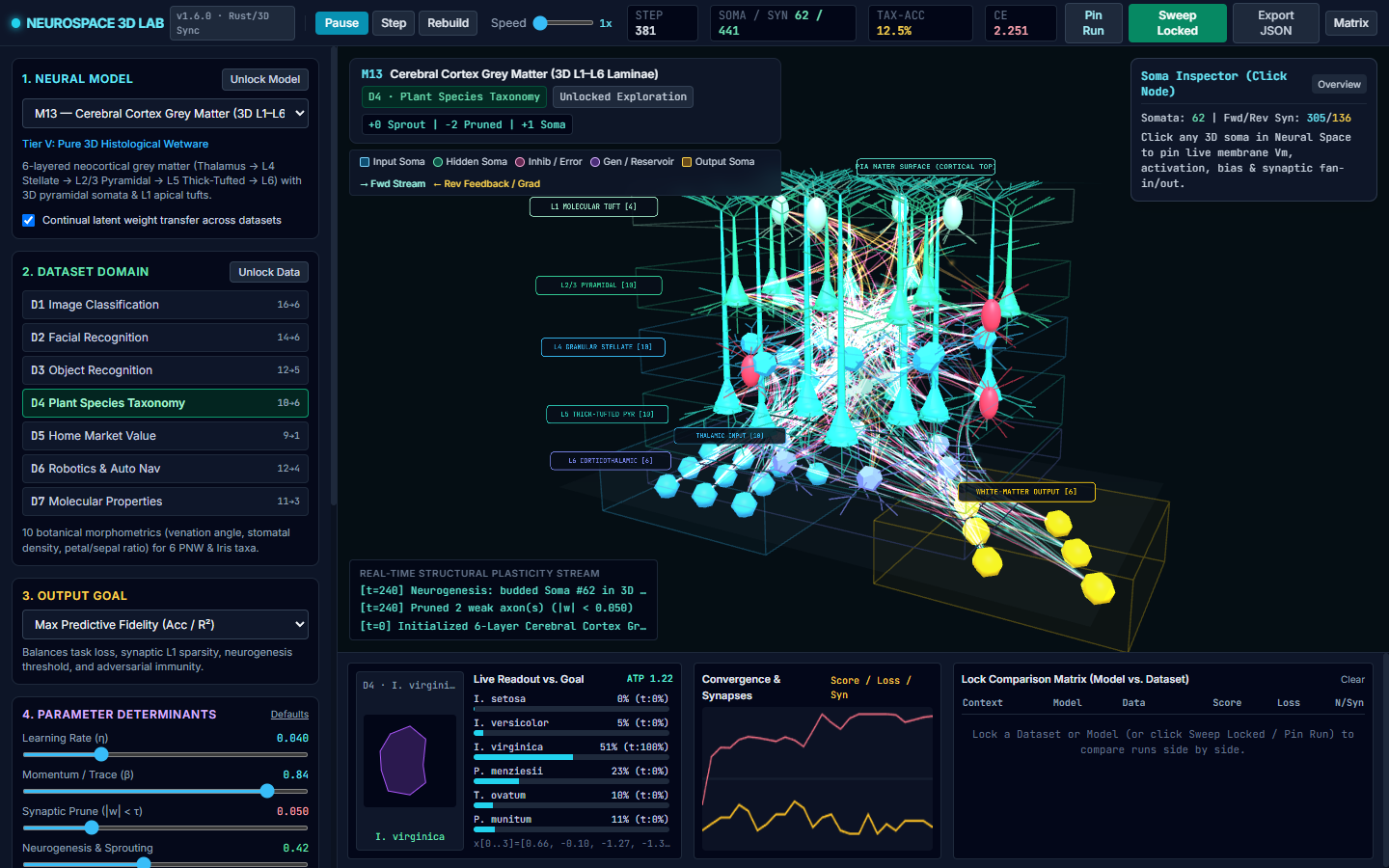
Static diagrams only tell part of the story: neural networks are dynamic, evolving graphs whose internal weights, active pathways, and structural connections shift continuously during training. To let researchers and students observe those dynamics directly, CRV Science developed NeuroSpace Lab (neurospace-lab v1.6.0), a safe-Rust 3D neural topology, structural plasticity, and cortical grey-matter workstation paired with a synchronized Three.js WebGL observatory. Across 15 selectable architectures—spanning classical perceptrons and deep MLPs up through sparse Transformers, Mixture-of-Experts language models, spiking LIF networks, and six-layered neocortical columns—NeuroSpace Lab renders live forward activation streams, reverse backpropagation counter-streams, synaptic pruning, neurogenesis, and side-by-side dataset benchmarking.
Discussion & Key Takeaways
Across six decades of research, neural networks succeeded not simply because computers grew faster, but because architectures evolved to reflect the real structure of scientific and perceptual data—spatial locality in vision, sequential memory in time series, flexible global context in Transformers, and relational bonds in Graph Neural Networks.
Pairing those architectural priors with simple stabilization tools (skip highways, normalization, and non-saturating activations) turned deep learning into a versatile foundation across science. Ongoing work now focuses on making these models reliable under distribution shift, well calibrated in their uncertainty, and faithful to physical laws.
References & Primary Sources
- [1] Rosenblatt, F. (1958). The perceptron: A probabilistic model for information storage and organization in the brain. Psychological Review. https://doi.org/10.1037/h0042519
- [2] Hopfield, J. J. (1982). Neural networks and physical systems with emergent collective computational abilities. Proceedings of the National Academy of Sciences. https://doi.org/10.1073/pnas.79.8.2554
- [3] Rumelhart, D. E., Hinton, G. E., & Williams, R. J. (1986). Learning representations by back-propagating errors. Nature. https://doi.org/10.1038/323533a0
- [4] Cybenko, G. (1989). Approximation by superpositions of a sigmoidal function. Mathematics of Control, Signals, and Systems. https://doi.org/10.1007/bf02551274
- [5] Hornik, K., Stinchcombe, M., & White, H. (1989). Multilayer feedforward networks are universal approximators. Neural Networks. https://doi.org/10.1016/0893-6080(89)90020-8
- [6] Hochreiter, S., & Schmidhuber, J. (1997). Long Short-Term Memory. Neural Computation. https://doi.org/10.1162/neco.1997.9.8.1735
- [7] LeCun, Y., Bottou, L., Bengio, Y., & Haffner, P. (1998). Gradient-based learning applied to document recognition. Proceedings of the IEEE. https://doi.org/10.1109/5.726791
- [8] Hinton, G. E., & Salakhutdinov, R. R. (2006). Reducing the Dimensionality of Data with Neural Networks. Science. https://doi.org/10.1126/science.1127647
- [9] Scarselli, F., Gori, M., Tsoi, A. C., Hagenbuchner, M., & Monfardini, G. (2009). The Graph Neural Network Model. IEEE Transactions on Neural Networks. https://doi.org/10.1109/tnn.2008.2005605
- [10] LeCun, Y., Bengio, Y., & Hinton, G. (2015). Deep learning. Nature. https://doi.org/10.1038/nature14539
- [11] He, K., Zhang, X., Ren, S., & Sun, J. (2016). Deep Residual Learning for Image Recognition. IEEE Conference on Computer Vision and Pattern Recognition (CVPR). https://doi.org/10.1109/cvpr.2016.90
- [12] Krizhevsky, A., Sutskever, I., & Hinton, G. E. (2017). ImageNet classification with deep convolutional neural networks. Communications of the ACM. https://doi.org/10.1145/3065386
- [13] Rawat, W., & Wang, Z. (2017). Deep Convolutional Neural Networks for Image Classification: A Comprehensive Review. Neural Computation. https://doi.org/10.1162/neco_a_00990
- [14] Belkin, M., Hsu, D., Ma, S., & Mandal, S. (2019). Reconciling modern machine-learning practice and the classical bias-variance trade-off. Proceedings of the National Academy of Sciences. https://doi.org/10.1073/pnas.1903070116
- [15] Jumper, J., et al. (2021). Highly accurate protein structure prediction with AlphaFold. Nature. https://doi.org/10.1038/s41586-021-03819-2